Index
1. Preface
KS integration (from Kelvin-Stokes integration) is a software that permits
lightcurve modelling in presence of stellar activity, able to account
for the photometric effect generated by transiting planets and
stellar spots, resolving also the cases in which these objects
appear overlapped with respect to the observer. It allows
spot merging and the creation of spot regions.
2. Licence
This program is free software: you can redistribute
it and/or modify it under the terms of the
GNU General Public License as published by the Free Software
Foundation, either version 3 of the License, or any later version.
This program is distributed in the hope that it will be useful, but WITHOUT ANY WARRANTY; without even the implied warranty of MERCHANTABILITY or FITNESS FOR A PARTICULAR PURPOSE. See the GNU General Public License for more details.
You should have received a copy of the GNU General Public License along with this program. If not, see http://www.gnu.org/licenses/
Contributed by M. Montalto, G. Boué, M. Oshagh, I. Boisse, G. Bruno, N. C. Santos
Copyright M. Montalto & Centro de Astrofísica, Universidade do Porto (CAUP)
3. Installation
The software is written in Fortran 95 and it has been tested
under a Linux machine using the GNU Fortran compiler gfortran.
The following instructions hold under the assumption that you
have this compiler already installed in your
machine. To proceed first unpack the tarfile:
tar -xvf KSint.tar.gz
this will create a directory KSint. Enter this directory and to create the executable type:
make
the executable KSint will be therefore found under the same directory. This program is a standalone program that works together with the input file 'inputs.txt' also located in the same directory as explained in the next Section.
In case you prefer to supply your own inputs in a different form or just want to incorporate this software in your own programs the main program under the SRC directory (KSint.f95) can be inspected. The subroutine that performs all the calculations is named KSflux.
4. Input file
Table 1 lists input parameters provided to the program
through the input file 'inputs.txt' in their order of
appearance. Input parameters are subdivided in four groups: SIMPARAM
contains parameters relative to the simulation, STARPARAM parameters
relative to the star, SPOTS and PLANETS relative to spots and planets
respectively as indicated by their name. For these two latter groups
the parameters relative to different planets (spots) are provided
as a comma separated list where it is only the number of planets and
spots declared by 'nplanets' and 'nspots' that will be considered during program
execution.
Table 1-Input parameters located in the file 'inputs.txt'.
Table 1-Input parameters located in the file 'inputs.txt'.
-
- Name
- Type
- Units
- Bounds
- Meaning
- SIMPARAM
-
- timestep
- REAL
- [days]
- >0.
- Timestep of each iteration
-
- nstep
- INTEGER
- -
- ≥1
- Total number of iterations
-
- nplanets
- INTEGER
- -
- ≥0
- Number of planets
-
- nspots
- INTEGER
- -
- ≥0
- Number of spots
- STARPARAM
-
- prot
- REAL
- [days]
- >0.
- Stellar rotation period
-
- incl
- REAL
- [degrees]
- [0.;180.]
- Stellar axis inclination
-
- posang
- REAL
- [degrees]
- [0.;360.]
- Position angle of stellar axis
-
- rho
- REAL
- [gcm-3]
- >0.
- Stellar density
-
- c1
- REAL
- -
- [0.;1.]
- Linear limb darkening coefficient
-
- c2
- REAL
- -
- [0.;1.]
- Quadratic limb darkening coefficient
- SPOTS
-
- lat
- REAL,REAL,...
- [degrees]
- [-90.;90.]
- Spots latitudes
-
- long
- REAL,REAL,...
- [degrees]
- [0.;360.]
- Spots longitudes
-
- adim
- REAL,REAL,...
- [degrees]
- ]0.;180.]
- Spots angular dimensions
-
- ffact
- REAL,REAL,...
- -
- ≠0,≤1.
- Spots contrast ratios
- PLANETS
-
- rp
- REAL,REAL,...
- -
- >0.
- Planets normalized radii
-
- porb
- REAL,REAL,...
- [days]
- >0.
- Planets orbital periods
-
- pincl
- REAL,REAL,...
- [degrees]
- [0.;180.]
- Planets orbital inclinations
-
- ecc
- REAL,REAL,...
- -
- [0.;1.[
- Planets orbital eccentricities
-
- w
- REAL,REAL,...
- [degrees]
- [0.;360.]
- Planets arguments of pericenters
-
- omega
- REAL,REAL,...
- [degrees]
- [0.;360.]
- Planets longitudes of the ascending nodes
-
- M
- REAL,REAL,...
- [degrees]
- [0.;360.]
- Planets initial mean anomalies
5. Reference systems
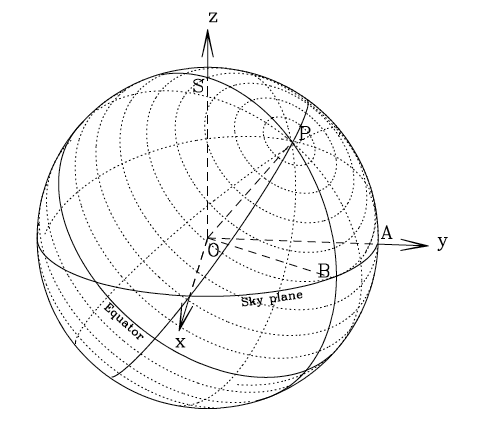
The angles introduced in Table 1 for planets and spots are
defined in Figure 1 and Figure 2.
The plane xy corresponds to the plane of the sky, while the z-axis is oriented towards the
observer.

Figure 1 - Star reference system.

In Figure 1, the star reference system is defined. The angle
between the North polar axis, from which the rotation is seen
counter-clockwise, and the line of sight (the arc SP) indicates the
inclination angle of the stellar axis (incl parameter). The angle
between the positive y-axis and the projection of the stellar axis to
the plane of the sky (the arc AB) is defined as the position angle of the
stellar axis (posang parameter). The latitude of a
spot (lat) is
defined along a stellar parallel from the equator, positive towardsthe
North pole. The longitude of a spot is measured along a stellar
meridian where the zero longitude meridian is the one passing through
the positive x-axis.
6. Overlapping spots
The present version of the code assumes the following rules once two or
more spots are overlapped: two or more spots with the same contrast ratio
will merge homogeneously (forming a region with the same contrast ratio of
the components), while two of more spots with different contrast ratios
will produce a region where the contrast ratio in the overlapping area
will be the sum of the contrast ratio of the components.
Note that it is not allowed to overlap two spots if the sum of their contrast ratios is larger than one.
7. Results
The results are stored by default in the file 'lc.dat'.
Optionally the program can reproduce the configuration of the system
at any given iteration. To enable this feature you should call the
program with the '-v niter' option where niter is the iteration number
you want to analyze. If the iteration number is not provided the
program will reproduce by default the first iteration configuration.
The result is stored in the file 'arcs.dat'.
The file 'lc.dat' contains three columns which correspond to the time of each iteration, the flux calculated by the program and an error flag which is equal to zero if no errors were detected.
The file 'arcs.dat' is separated in three different sections. The first line provides the starting, final lines in the file relative to the ARCS section, and in the last column provides the number of objects to which the arcs belong. The second line provides the starting, final lines in the file relative to the stellar GRID section, and the third line gives the starting line of the ROOTS section.
All the coordinates reported below are expressed with respect to the XY observer plane.
The ARCS section provides the coordinates x, y of each point on a given arc, followed by a flag which is one if that point lies on an integrable arc, and by a number which is unique for each object (one corresponds by default to the stellar border). The GRID section gives the x, y coordinates of each point on a stellar parallel or meridian. The third column is just an incremental number running along the maximum circles, while the last column is a flag which is equal to one in the case the point belongs to a parallel, two if it belongs to a meridian and zero if it lies on the invisible hemisphere of the star. The ROOTS section gives the x, y coordinates of the arcs interception points found by the root finding algorithm. A fully integrable object has always a root attributed to the arc defining its profile, since the arc is integrated between zero and 2π.
Under the directory SM and GNUPLOT simple macros are provided and can be used to visualize the results in 'lc.dat' and 'arcs.dat'.
Additionally, once the '-v niter' option is used an arc table is printed on the screen, showing, for each object, the list of arcs splitting the profile of each object. The starting and final angles of the arc are reported in the first and second columns respectively. For the case of planets and the case of the stellar border, the angle is counted counter-clockwise from the positive x-axis with respect to a reference system centered on each object and with the axis oriented like the observer XY reference system. For the case of spots the angle α is reported as defined in Fig. 1 of the paper. The third column gives the contrast ratio associated to the arc (this is the factor that multiplies the integral on that arc, resulting from the analysis of the structure), while the fourth column is a flag indicating if the arc is considered integrable (in this case the flag is equal to one).
8. Example
The following example may be used as a guide to get started
using the program.
We simulate the case of a planet crossing a naked eye
spot. The input parameters are provided in Table2.
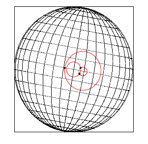
The resulting configuration (as seen by the observer) at iteration 833 of
the simulation is shown in Figure 3. Here the positive x-axis is
oriented towards the right while the positive y-axis towards the top.
The resulting lightcurve is shown in Figure 4.
-
Table 2-Input parameters relative to the example
-
- Name
- Value
- SIMPARAM
-
- timestep
- 0.0009
-
- nstep
- 1000
-
- nplanets
- 1
-
- nspots
- 2
- STARPARAM
-
- prot
- 30.
-
- incl
- 90.
-
- posang
- 10.
-
- rho
- 0.4
-
- c1
- 0.4
-
- c2
- 0.3
- SPOTS
-
- lat
- 0.2,-0.3
-
- long
- 270.2,270.
-
- adim
- 18.,4.
-
- ffact
- 0.1,0.8
- PLANETS
-
- rp
- 0.12
-
- porb
- 3.
-
- pincl
- 90.
-
- ecc
- 0.
-
- w
- 0.
-
- omega
- 180.
-
- M
- 0.
discussed in the text.
Figure 3 - Planet overlapped with a naked eye spot at iteration 833 of the example.


Figure 4 - This Figure shows a portion of the resulting lightcurve where the planet overlaps the spots.


9. Credits
The KS technique applied to the case of planets and spots is discussed
in the two following papers:
Pál, A. 2012, MNRAS, 420, 1630
Montalto, M., Boué, G., Oshagh, M., Boisse, I., Bruno, G., Santos, N. C. 2014, MNRAS, 444, 1721
The solution presented in this software incorporates the one on planets presented in Pál, therefore any work where this software is used should mention these two papers.
Pál, A. 2012, MNRAS, 420, 1630
Montalto, M., Boué, G., Oshagh, M., Boisse, I., Bruno, G., Santos, N. C. 2014, MNRAS, 444, 1721
The solution presented in this software incorporates the one on planets presented in Pál, therefore any work where this software is used should mention these two papers.


